WHIR: Super-Fast Verification for Hash-Based SNARKs

What problem are we solving?

If you’ve followed hash-based SNARGs over the last few years — FRI, STIR, BaseFold, Brakedown — you’ve watched the field push hard on prover time, proof size, and post-quantum security. The one cost that didn’t move much was verifier time. Verifying a hash-based SNARG typically takes a few milliseconds, with most of that going to field arithmetic against the verifier’s challenges. A few milliseconds sounds fine until you remember the two settings that matter most:

• On-chain verifiers pay gas per field operation. Every millisecond is dollars.
• Recursive provers verify a SNARG inside their next SNARG. The verifier cost becomes part of the next prover’s circuit — and shrinking it shrinks the next proof too.

WHIR (Arnon, Chiesa, Fenzi, Yogev — 2024) is a new IOP of proximity that drops hash-based SNARG verification into the few-hundred-microseconds regime. The paper’s abstract example, at $2^{22}$ coefficients, rate $1/4$, and 100 bits of security, reports commit + open in 1.2 seconds, proof size 63 KiB, and verification in 360 µs.

To compare against prior work on a setting where everyone has data — $m = 24$, $\rho = 1/2$, 100 bits of security — WHIR-CB verifies in 0.61 ms vs BaseFold’s 24 ms (a $39\times$ gap). At 128 bits of security on a 192-bit prime field, WHIR-CB verifies in 1.0 ms vs STIR’s 3.8 ms and FRI’s 3.9 ms.

Underneath that headline are two ideas worth understanding:

1. Constrained Reed–Solomon codes (CRS). A small generalization of the Reed–Solomon code that bundles a polynomial code with a sumcheck-style constraint. CRS turns out to be the right object to test against — one IOPP for CRS gives you a low-degree test, a polynomial commitment opening, and a sumcheck query checker, all in one protocol.

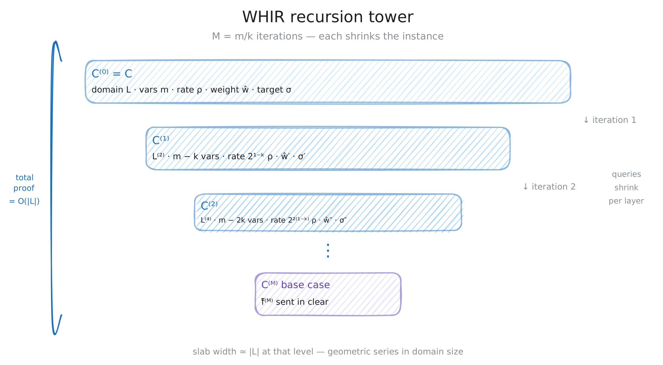
2. Sumcheck-inside-the-IOPP. Each WHIR iteration runs a few rounds of sumcheck on $f$, then folds $f$, then samples the folded function out-of-domain, then queries it at a few shift points — and packs all of that into the constraint of a smaller CRS instance. The recursion drives $m$ (number of variables) down by $k$ each iteration while halving the domain.

The verifier-cost shape, in plain words: roughly $\lambda$ queries, each touching a small fold neighborhood and updating one constraint. Same query count as STIR, but each query is much cheaper to handle — concrete formulas in the table below.

The article walks through the protocol, the design choices that make it fast, and how the same machinery yields a polynomial commitment for free.

Prerequisites. Comfort with multilinear polynomials, the sumcheck protocol, Reed–Solomon codes, and the rough shape of FRI-style IOPPs. We’ll set up the rest from scratch.

Headline numbers and the comparison table

Before touching the protocol, here is the headline comparison from the paper (Table 1, paraphrased). The dependence on rate $\rho$ is suppressed:

Two things to notice:

• WHIR matches STIR on query count. Both have the same logarithmic dependence on $m$, both crush BaseFold’s linear-in-$m$ count.
• WHIR’s verifier time is smaller than STIR’s. Compare the two formulas: STIR pays $q \cdot 2^k$ plus an additive $\frac{\lambda^2}{k} \cdot 2^k$ overhead from its quotient bookkeeping. WHIR pays $q \cdot (2^k + m)$ — no quotient term. The $+m$ inside the per-query cost is the sumcheck-verification-and-eq-evaluation work, which is cheap.

That second row is the entire reason WHIR’s verifier breaks into the microsecond regime.

Background

Three concepts do most of the lifting: smooth Reed–Solomon codes (and their multilinear view), folding, and the IOP-of-proximity abstraction. One quick notation reminder before we dig in:

So $\mathsf{RS}[\mathbb F, L, m]$ is a code where messages have $2^m$ coefficients and codewords have $\lvert L \rvert$ field elements. Sumcheck operates on the message side (sums over the boolean hypercube $\{0,1\}^m$, size $2^m$), not on the codeword side. The codeword on $L$ is a redundant encoding of the message — you don’t sum over the encoding, you sum over the message it encodes.

Smooth Reed–Solomon codes, two ways

WHIR uses smooth Reed–Solomon codes. Reed–Solomon itself is a prereq — if it’s rusty, Thaler’s PAZK book chapter on low-degree testing is a clean refresher. This section focuses on what smoothness adds and why WHIR needs it.

$L$ is smooth when it’s a multiplicative coset of $\mathbb F^\ast$ whose order is a power of two. The interesting consequence — and the reason WHIR needs it — is that smoothness lets squaring halve the domain cleanly, repeatedly, all the way down. Three properties of a smooth $L$ chain together to make this work:

1. $-1 \in L$. A cyclic group of even order over a field of characteristic $\neq 2$ contains a unique element of order 2 — that’s $-1$.
2. $L$ closed under negation. Once $-1 \in L$, multiplying any $x \in L$ by $-1$ stays inside (cosets are closed under multiplication by subgroup elements). So elements pair up under $x \leftrightarrow -x$.
3. Squaring collapses each pair. $x^2 = (-x)^2$, so the squaring map sends both members of every pair to the same image. The image set $L^{(2)} := \{x^2 : x \in L\}$ has exactly half the elements.

A concrete example makes the chain easy to see. Pick $\mathbb F_{17}$. Its multiplicative group has order $16 = 2^4$, so it’s smooth. Take the order-8 subgroup:

Property 1 lands: $L$‘s order is 8 (even), and indeed $16 \equiv -1 \pmod{17}$ is in $L$. Property 2 follows: pairs under negation $(x, -x = 17-x)$ are $(1, 16), (2, 15), (4, 13), (8, 9)$ — every pair sits inside $L$. And property 3 collapses them under squaring:

Distinct images: $L^{(2)} = \{1, 4, 13, 16\}$ — half the size, as promised. The same three properties hold for $L^{(2)}$ (still a power-of-two-order coset), so squaring halves again: $L^{(4)} = \{1, 16\}$, then $L^{(8)} = \{1\}$. After $\log_2 |L|$ squarings the set is exhausted.

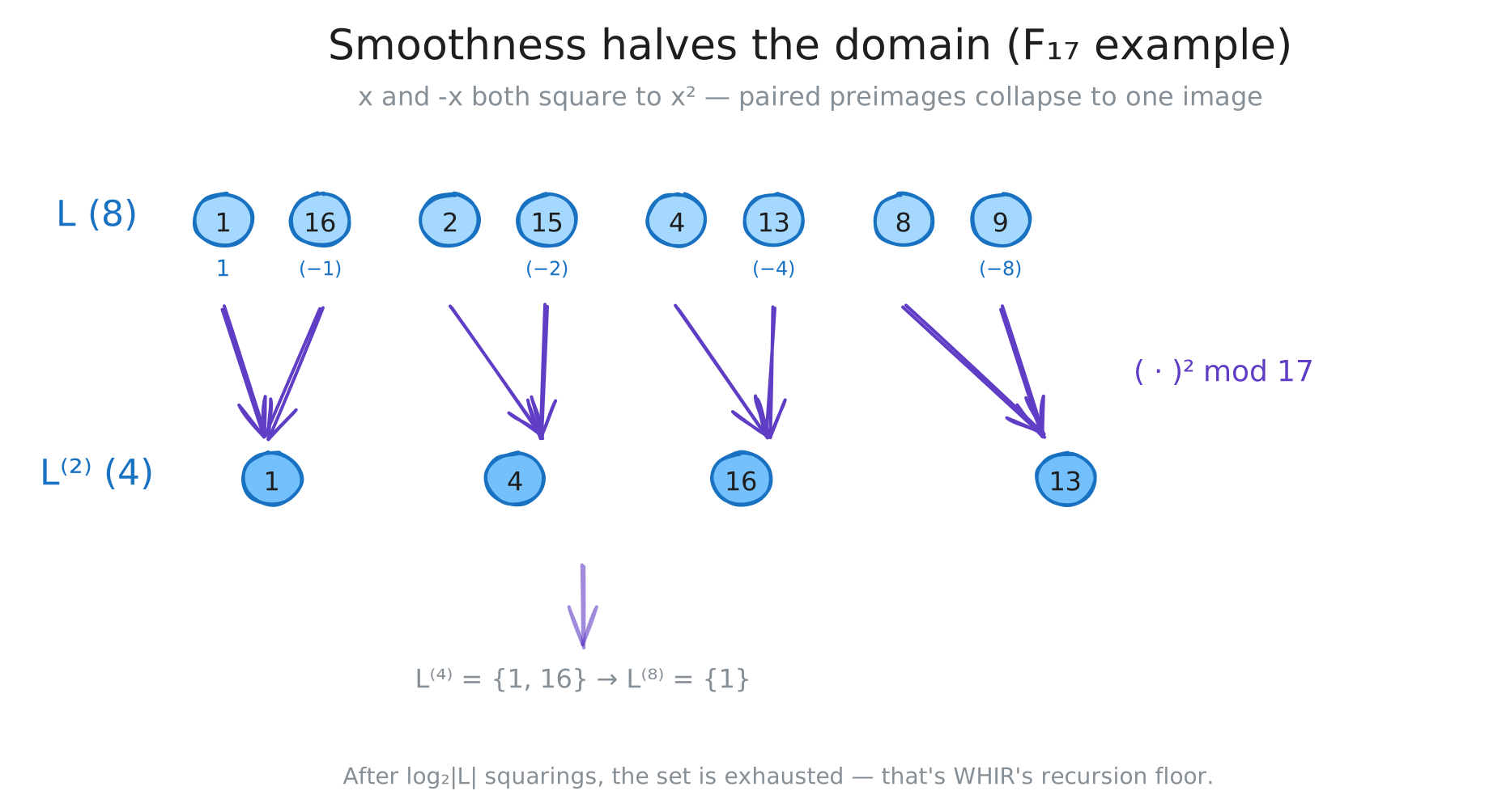
This iterated halving is what powers WHIR’s recursion: each iteration squares $L$ once and shrinks the multilinear $\hat f$ by binding several of its variables to verifier randomness.

Why smoothness matters: two readings of the same vector.

A Reed–Solomon codeword is just a vector of $|L|$ field values. Once $L$ is smooth, that exact vector admits two completely different polynomial interpretations — and WHIR uses both, switching lenses mid-protocol.

Reading 1 — univariate. The vector is the evaluations of a single univariate polynomial $\hat g$ of degree $< 2^m$, one value per point of $L$. This is the FRI-world reading: low-degree testing and folding live here.

Reading 2 — multilinear. The same vector is the evaluations of a multilinear polynomial $\hat f$ in $m$ variables. To evaluate, you don’t plug in one number — you plug in $m$ numbers. Specifically, for each $x \in L$, plug $\hat f(x, x^2, x^4, \ldots, x^{2^{m-1}})$. So one univariate input $x$ gets stretched into an $m$-tuple by squaring. This is the BaseFold/Spartan reading: sumcheck lives here.

The two readings encode the same coefficient data. The clearest way to see why is to work out the smallest non-trivial case, $m = 2$.

A degree-3 univariate has 4 coefficients:

A multilinear in 2 variables also has 4 coefficients — one per subset of $\{X_1, X_2\}$:

Now substitute $X_1 = x$ and $X_2 = x^2$ — that’s the smoothness curve at $m=2$:

Match coefficients with $\hat g$: $a_0 = b_0$, $a_1 = b_1$, $a_2 = b_2$, $a_3 = b_3$. Same numbers, just relabeled. And there’s a clean rule for the relabeling: the coefficient of $X^k$ in the univariate matches the multilinear coefficient whose variable subset is given by the binary expansion of $k$. Index 3 in binary is $11$, picking $\{X_1, X_2\}$, giving the monomial $X_1 X_2 = x \cdot x^2 = x^3$. Each bit of $k$ tells you whether to include the corresponding variable.

This generalizes: for any $m$, plugging $X_i := x^{2^{i-1}}$ into the multilinear and expanding reassembles the univariate, term by term. Smoothness ensures the substitution evaluates correctly at every point of $L$:

Why we care. WHIR uses folding from the univariate reading and sumcheck from the multilinear reading. The protocol runs sumcheck on $\hat f$ (Reading 2), then folds the result (Reading 1) — and the smoothness curve is the bridge that lets a single object switch lenses mid-protocol. The two operations are gear-meshed by the curve: the verifier randomness $\boldsymbol\alpha$ generated by sumcheck (binding the multilinear’s variables) is the same $\boldsymbol\alpha$ used to fold the univariate vector. Claim 4.15 of the paper makes this exact: the univariate fold equals the multilinear restriction $\hat f(\boldsymbol\alpha, X_{k+1}, \ldots, X_m)$.

One naming convention for the road: when you have a univariate point $z$ and the multilinear reading needs an $m$-dimensional evaluation point, the lift $\mathbf z := (z, z^2, z^4, \ldots, z^{2^{m-1}})$ hands it to you — just $z$ run through the smoothness curve. Univariate-at-$z$ equals multilinear-at-$\mathbf z$.

This dual view is the bridge between FRI-world (univariate, low-degree testing) and BaseFold-world (multilinear, sumcheck).

Folding

Folding is FRI’s signature move. Picture it as shrinking the code in half with verifier randomness as the lever.

You start with $f$, a vector of $|L|$ values. After folding with a verifier-supplied randomness $\alpha$, you get $\mathsf{Fold}(f, \alpha)$, a new vector of $|L|/2$ values laid out on the squared domain $L^{(2)} := \{x^2 : x \in L\}$. The crucial property: if $f$ was an RS codeword for some degree-$<2^m$ polynomial, the folded vector is itself an RS codeword — for some new degree-$<2^{m-1}$ polynomial. Folding doesn’t just shrink the vector; it shrinks the underlying polynomial too.

The recipe: each entry of the folded vector is a randomized mixture of two paired entries of the original. For each $y \in L^{(2)}$ there are exactly two values in $L$ that square to $y$ — the pair $x$ and $-x$ from the previous section. Take the values of $f$ at this pair, mix them with $\alpha$:

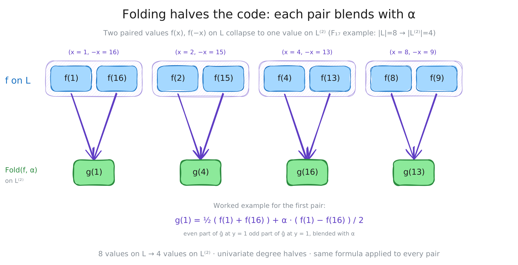
Why this particular formula? Split the underlying univariate polynomial $\hat g$ into even and odd parts: $\hat g(X) = \hat g_{\text{even}}(X^2) + X \cdot \hat g_{\text{odd}}(X^2)$. Then $f(x) + f(-x) = 2 \hat g_{\text{even}}(x^2)$ (the odd part cancels) and $f(x) - f(-x) = 2x \cdot \hat g_{\text{odd}}(x^2)$ (the even part cancels). So sum-of-pair extracts the even coefficients; scaled-difference-of-pair extracts the odd ones. Mixing them with $\alpha$ gives a new polynomial $\hat g_{\text{even}}(Y) + \alpha \cdot \hat g_{\text{odd}}(Y)$ in the squared variable $Y = x^2$ — a polynomial of half the original degree, evaluated on the half-sized domain $L^{(2)}$.

There’s a clean polynomial identity that makes this exact. Write $\hat f$ split by its first variable: $\hat f(X_1, X_2, \ldots, X_m) = \hat f_0(X_2, \ldots) + X_1 \cdot \hat f_1(X_2, \ldots)$. Folding with $\alpha$ is the same as plugging $\alpha$ in for $X_1$:

In one sentence: folding with $\alpha$ binds the first variable of $\hat f$ to $\alpha$. The code goes from $\mathsf{RS}[\mathbb F, L, m]$ to $\mathsf{RS}[\mathbb F, L^{(2)}, m-1]$ — the domain is halved and the polynomial loses one variable.

We’ll iterate folding $k$ times with a vector of randomness $\boldsymbol\alpha = (\alpha_1, \ldots, \alpha_k) \in \mathbb F^k$, written $\mathsf{Fold}(f, \boldsymbol\alpha) : L^{(2^k)} \to \mathbb F$. To compute one entry of the $k$-fold result, the verifier needs the $2^k$ values of $f$ at the $2^k$-th roots of a single point — $O(2^k)$ field operations, using a coefficient-encoding trick the paper exploits.

Distance preservation. Folding’s soundness property: if $f$ is $\delta$-far from $\mathsf{RS}[\mathbb F, L, m]$ (i.e., disagrees with every codeword on a $\delta$-fraction of positions), then $\mathsf{Fold}(f, \alpha)$ stays $\delta$-far from $\mathsf{RS}[\mathbb F, L^{(2)}, m-1]$ with high probability over $\alpha$. Verifier randomness keeps the distance from collapsing — without it, a sneaky prover could fold a non-codeword into something that looks like a codeword. This soundness fact is correlated agreement for Reed–Solomon, the [BCIKS20] result that powers FRI/STIR/WHIR’s analyses.

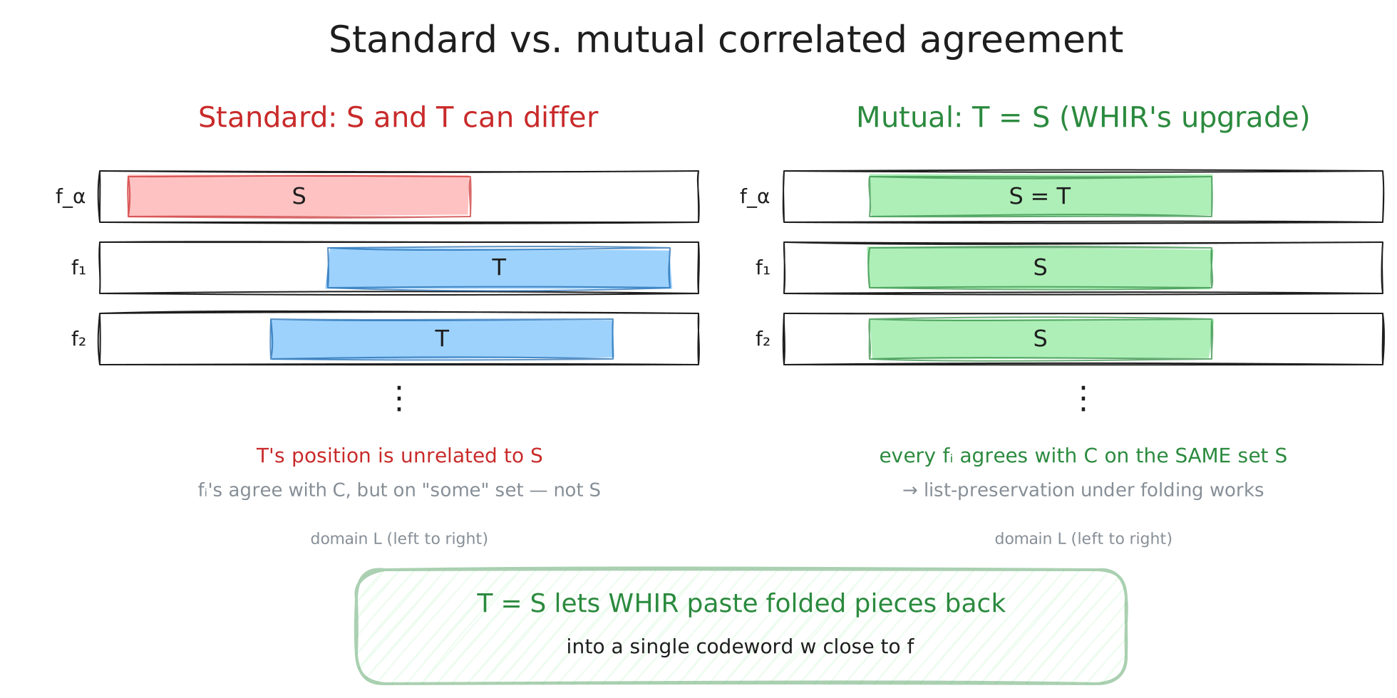
WHIR needs a slightly stronger version — mutual correlated agreement, which insists not just that the components agree with codewords somewhere but on the same set. We unpack why that sameness matters in §Idea 2.

IOPs of proximity

When we describe WHIR in detail, there’s a lot of mechanical plumbing — Merkle trees, hashes, Fiat–Shamir. We abstract that away. An IOP of proximity (IOPP) for a code $C$ is a protocol where:

• The prover sends an oracle $f : L \to \mathbb F$ (think: a long vector).
• The verifier issues some random challenges and reads a small number of entries of $f$ (point queries) plus possibly more oracles.
• The verifier accepts if $f$ is close to $C$, rejects if it’s far.

The compilation to a real hash-based protocol is mechanical (BCS transform): commit each oracle via a Merkle tree, send Merkle paths instead of point answers, hash everything for Fiat–Shamir. The number of point queries equals the number of Merkle paths in the final SNARG, so query count is a real cost.

Idea 1 — Constrained Reed–Solomon codes

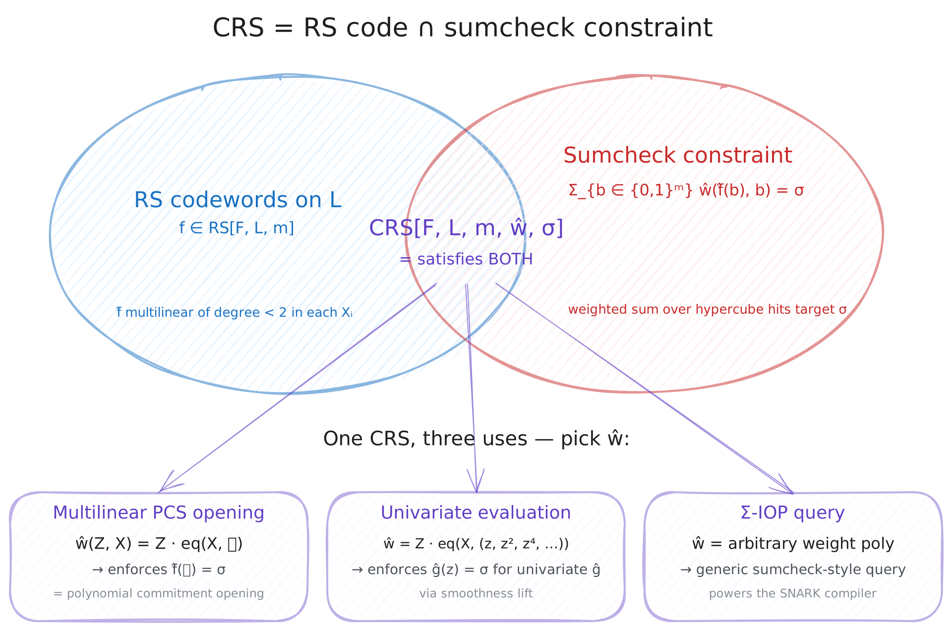
The move. Take a Reed–Solomon code and also require that some weighted sum of the codeword’s values over the boolean cube equals a target $\sigma$. The sum-shaped extra slot is rich enough to encode “this codeword evaluates to $y$ at point $\mathbf z$” or “this codeword satisfies a sumcheck-style query” as a single membership question — so checking proximity to a CRS code is the PCS opening, is the sumcheck residue check, is the Σ-IOP query.

Formally, a constrained Reed–Solomon code is a Reed–Solomon code plus an extra sumcheck-style constraint on the underlying multilinear polynomial:

The weight polynomial $\hat w(Z, X_1, \ldots, X_m)$ is a polynomial in $m+1$ variables. The target $\sigma \in \mathbb F$ is the value the sum has to hit. A codeword $f$ has to (a) be a Reed–Solomon codeword in the usual sense, and (b) satisfy the sum constraint when you expand it as a multilinear $\hat f$.

That’s the whole definition. The trick is what you can encode in $\hat w$:

• Point evaluation. Set $\hat w(Z, X) := Z \cdot \mathsf{eq}(X, \mathbf z)$ for a target point $\mathbf z \in \mathbb F^m$. Here $\mathsf{eq}$ is the multilinear extension of boolean equality — picture it as a selector that’s $1$ when $b = \mathbf z$ on the cube and $0$ on every other cube point. Concretely, $\mathsf{eq}(b, \mathbf z) = \prod_i (b_i z_i + (1-b_i)(1-z_i))$. Then:

  $$\sum_{b \in \{0,1\}^m} \hat w\big(\hat f(b), b\big) = \sum_b \hat f(b) \cdot \mathsf{eq}(b, \mathbf z) = \hat f(\mathbf z)$$

  So $\sigma = \hat f(\mathbf z)$. The CRS code carves out, from all RS codewords, those whose multilinear evaluates to $\sigma$ at $\mathbf z$. This is exactly a polynomial commitment opening. The IOPP for this CRS code, compiled, is a multilinear PCS.

• Univariate evaluation. A univariate polynomial of degree $<2^m$ evaluated at $z \in \mathbb F$ corresponds, via the smoothness identity, to evaluating its multilinear at $\mathbf z = (z, z^2, z^4, \ldots, z^{2^{m-1}})$. So univariate point evaluations are CRS too.

• Arbitrary sumcheck-like queries. Any polynomial $\hat w$ that’s cheap to evaluate gives a valid query. This is what makes WHIR usable as the proximity-test backbone of a Σ-IOP compiler — a poly-IOP variant where the verifier asks weighted-sum queries instead of single-point evaluations, covered later in this article.

The punchline: CRS unifies “test that $f$ is a Reed–Solomon codeword” with “test that $\hat f$ takes a specific value at a specific place.” Both are CRS proximity tests. Build one good IOPP for CRS, and you get the proximity test, the PCS, and the Σ-IOP query mechanism in one shot.

What the verifier actually sees

Before the protocol walk, anchor on what’s actually on the wire. The verifier never inspects $\hat f$ in full — it only sees a few Merkle roots, sumcheck messages, and a handful of opened entries.

Commit phase. The prover takes the multilinear $\hat f$, encodes it as $f : L \to \mathbb F$ via the smoothness curve, Merkle-commits the $\lvert L \rvert$ entries of $f$, and sends one root hash to the verifier. That hash is the entire commitment.

Open phase, per WHIR iteration. For an opening claim like $\hat f(\mathbf z) = \sigma$, each iteration puts the following on the wire:

• $k$ sumcheck messages $\hat h_1, \ldots, \hat h_k$ — small univariate polynomials.
• A new Merkle root for the folded oracle $g : L^{(2)} \to \mathbb F$.
• One OOD answer $y_0 \in \mathbb F$.
• $t$ shift-query answers — for each $z_i$, the $2^k$ values of $f$ at the $2^k$-th roots of $z_i$, plus a Merkle path proving they came from the committed root.

After $M = m/k$ iterations, the prover sends the final small multilinear $\hat f^{(M)}$ in the clear (constant size). That’s the only point where the verifier sees a real polynomial.

How binding works. The verifier never directly checks “is the prover using the same $\hat f$ in sumcheck as in the codeword?” Instead, it runs a chain of independent gates. To cheat, the prover has to break every gate simultaneously:

If every gate passes, the soundness analysis says: with overwhelming probability there exists a single multilinear $\hat f$ such that the committed $f$ encodes it AND the original opening claim $\hat f(\mathbf z) = \sigma$ holds. The verifier doesn’t need to see $\hat f$ — it just needs the prover to be unable to lie consistently across all the gates at once.

The WHIR iteration

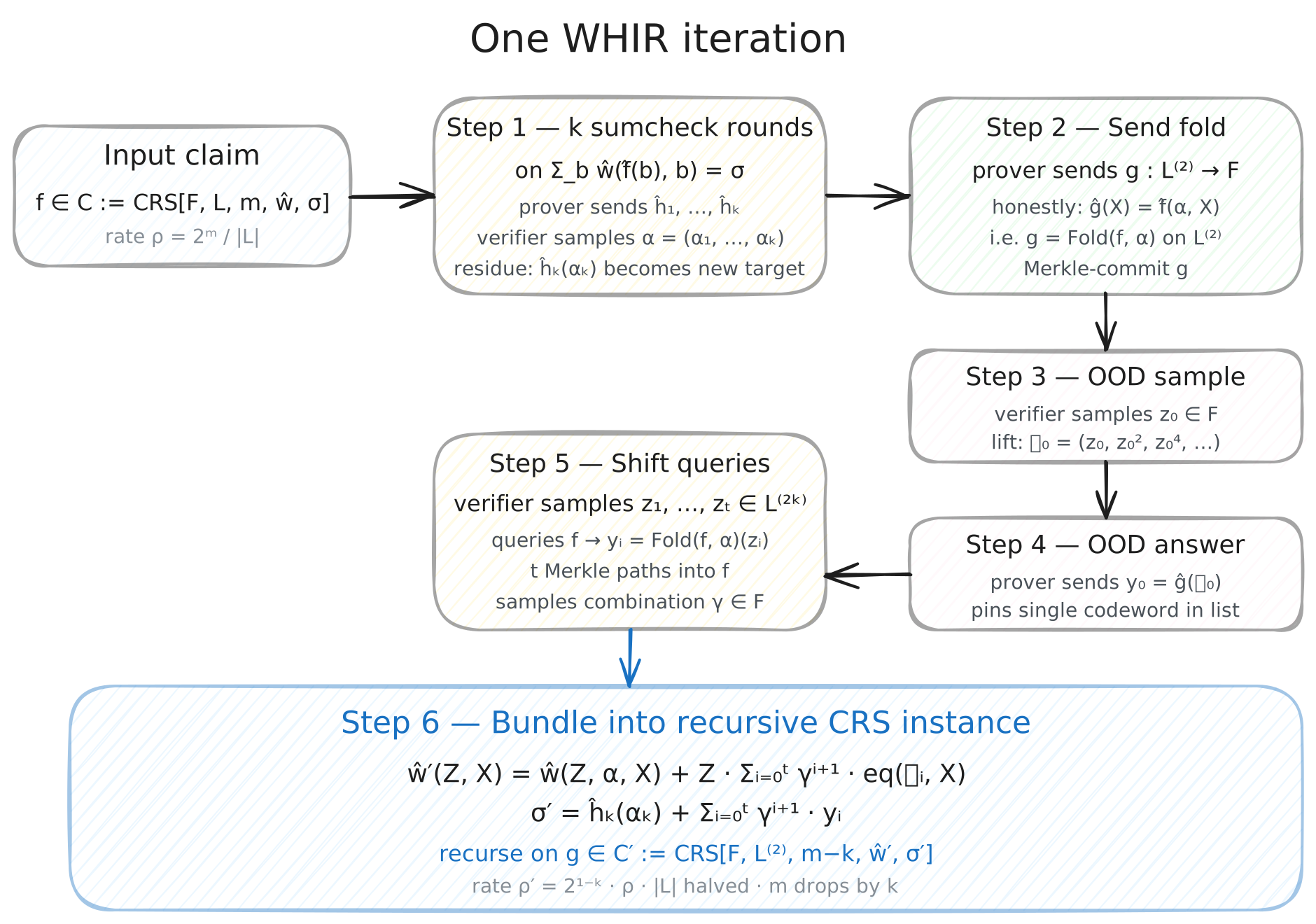
Now the protocol. We describe one iteration of WHIR. The iteration reduces testing

to testing

for some new weight polynomial $\hat w'$ and target $\sigma'$ that the protocol constructs along the way. The full protocol applies $M = m/k$ iterations until $C^{(M)}$ has only a few variables left and the prover sends $\hat f^{(M)}$ in the clear.

For this overview, assume $\hat w$ is multilinear (the paper handles a more general setting).

Step 1 — $k$ rounds of sumcheck

The move: burn down $k$ of the $m$ variables in the CRS constraint via sumcheck. After $k$ rounds, the first $k$ variables of $\hat f$ are pinned to verifier randomness $\boldsymbol\alpha$, and the leftover sum is over $m-k$ variables. The new target — the one the recursive instance has to hit — is whatever the sumcheck protocol leaves on the table.

Concretely, prover and verifier run sumcheck on the constraint built into $C$. After $k$ rounds, the prover has sent $k$ univariate polynomials $\hat h_1, \ldots, \hat h_k$ (one per round) and the verifier has sampled $\boldsymbol\alpha = (\alpha_1, \ldots, \alpha_k)$. The remaining claim is the partially-bound sum:

The verifier knows $\hat h_k(\alpha_k)$ — they checked the round-by-round sumcheck equations. What they don’t yet know is whether the prover’s sumcheck polynomials are consistent with the actual $\hat f$. That’s the verifier’s eventual job, and the rest of the iteration is structured to feed exactly that check into the recursive instance.

Step 2 — Send the folded function

The purpose: hand the verifier a smaller object to recurse on. After Step 1’s sumcheck rounds, the multilinear has $m-k$ free variables left; the prover commits to its evaluations on the half-sized domain $L^{(2)}$. That’s the new RS codeword the recursive instance will check.

How: the prover sends $g : L^{(2)} \to \mathbb F$ as a fresh Merkle-committed oracle. Honestly, $g$ is the evaluation on $L^{(2)}$ of the multilinear $\hat g(X) := \hat f(\boldsymbol\alpha, X)$ — the same multilinear as the iterated fold $\mathsf{Fold}(f, \boldsymbol\alpha)$, but encoded on the bigger domain $L^{(2)}$ instead of $L^{(2^k)}$ (where the iterated fold would naturally land). For $k = 1$ these coincide; for $k > 1$, $g$ is a more redundant encoding of the same polynomial.

Note the asymmetry. Step 1 bound $k$ variables of $\hat f$ on the multilinear side, but Step 2 only halves the domain once on the codeword side. The new codeword $g$ has length $\lvert L \rvert / 2$, not $\lvert L \rvert / 2^k$ — bigger than the minimum needed. The polynomial it encodes ($\hat g$ with $m-k$ variables, $2^{m-k}$ coefficients) fits comfortably in this larger domain, with room to spare for parity. This is deliberate: the new code becomes lower-rate (more redundant), and lower rate buys query savings on the recursive instance. We make this precise in §“Why the rate decreases”.

The verifier doesn’t trust $g$ yet. The next steps are what tie it back to $f$.

Step 3 — Out-of-domain round

The purpose: pin down a single codeword as “the” $g$, even when list decoding leaves many candidates. Beyond the unique-decoding radius, several distinct codewords can sit within distance $\delta$ of the prover’s claimed $g$ — that’s “the list.” Without OOD, the soundness analysis would have to track every codeword in the list, which is a mess. OOD forces the prover to commit to a single multilinear by binding its evaluation at a fresh random point outside $L^{(2)}$.

How: the verifier samples $z_0 \leftarrow \mathbb F$ (out-of-domain — that’s the “OOD”) and sends it. Set $\mathbf z_0 := \mathsf{pow}(z_0, m-k) = (z_0, z_0^2, z_0^4, \ldots)$ — the smoothness lift of $z_0$. The prover replies with $y_0 \in \mathbb F$, which honestly is $\hat g(\mathbf z_0)$.

Why one codeword wins. At most one codeword $\hat u$ in the list can satisfy $\hat u(\mathbf z_0) = y_0$, because two distinct multilinear polynomials disagree at a random point with probability close to 1 (Schwartz–Zippel). So OOD picks out a single codeword to call “the” $g$ — same trick DEEP-FRI [BGKS20] introduced for FRI; WHIR reuses it inside every iteration.

Deferred verification. The verifier doesn’t actually check $y_0$ at this step. The value $y_0$ flows into $\sigma'$ in Step 5; the recursive CRS check is what enforces $\hat g(\mathbf z_0) = y_0$ later, together with everything else. Step 3 gathers the OOD claim; it doesn’t verify it.

Step 4 — Shift queries

The purpose: force the prover’s claimed $g$ to actually agree with the fold of the committed $f$ on $t$ random spot checks. Without these, a cheating prover could send any $g$ that satisfies the OOD claim and walk away. The shift queries are the only place in the entire iteration where the verifier directly reads from $f$ — every other check operates on the fresh oracle $g$ or on small messages.

The mechanics. Verifier samples $z_1, \ldots, z_t \leftarrow L^{(2^k)}$, lifts each to $\mathbf z_i := \mathsf{pow}(z_i, m-k)$, and samples a combination randomness $\gamma \leftarrow \mathbb F$. For each $z_i$, the verifier needs to compute $y_i := \mathsf{Fold}(f, \boldsymbol\alpha)(z_i)$ — the value of the iterated $k$-fold of $f$ at the point $z_i$. The verifier only has a Merkle commitment to $f$, not the full vector. How does it compute the fold from queries alone?

The $2^k$-th roots and the local fold. The “$2^k$-th roots of $z_i$” are the $2^k$-many $x \in L$ such that $x^{2^k} = z_i$. Two facts about smoothness make this exact count work:

• Squaring is 2-to-1 on a smooth domain (each $y \in L^{(2)}$ has two preimages $\pm x$ in $L$). Iterating $k$ squarings is $2^k$-to-1 — every point of $L^{(2^k)}$ has exactly $2^k$ preimages back in the original domain $L$.
• Smoothness guarantees these preimages all live inside the committed domain $L$ (no need to extend). They’re the leaves the verifier can ask for via Merkle paths.

The verifier reads only those $2^k$ values of $f$ — typically with one Merkle path, since the prover lays out $f$‘s tree so that all $2^k$ preimages of any $L^{(2^k)}$ point sit in adjacent leaves (a single path opens the whole leaf cluster). Plug them into the iterated fold formula (the recipe from §Folding, applied $k$ times via $\boldsymbol\alpha = (\alpha_1, \ldots, \alpha_k)$) and you get one value $y_i = \mathsf{Fold}(f, \boldsymbol\alpha)(z_i)$ — computed locally, in $O(2^k)$ field operations. The verifier never folds the entire $f$; it folds only at the sampled points.

Total cost: $t$ Merkle paths into $f$, one per $z_i$, each opening $2^k$ adjacent positions.

Deferred verification. The $y_i$ values aren’t compared to $g$ directly at this step. They flow into $\sigma'$ in Step 5; the recursive CRS check is what enforces ”$\hat g(\mathbf z_i) = y_i$ for every $i$.” If $g$ wasn’t actually close to the fold of $f$, at least one $\mathbf z_i$ likely lands where the recursive check fails — but that failure surfaces during recursion, not here.

Step 5 — Recursive claim

The trick. The verifier has accumulated three open obligations: the sumcheck residue from Step 1, the OOD claim from Step 3, and the $t$ shift-query claims from Step 4. Rather than discharge them externally — quotient polynomials, side checks, extended-domain bookkeeping — WHIR welds all three into the constraint of a smaller CRS instance and recurses on that single object. The CRS slot is rich enough to absorb every accumulated check, so the protocol moves on with one obligation, not three.

Concretely, define a new weight polynomial $\hat w'$ and new target $\sigma'$:

The new constraint $\hat w'$ packs three things into one CRS instance:

• The sumcheck residue from Step 1 ($\hat w(Z, \boldsymbol\alpha, X)$ with target $\hat h_k(\alpha_k)$).
• The OOD constraint from Step 3 (the $i = 0$ term: $Z \cdot \gamma \cdot \mathsf{eq}(\mathbf z_0, X)$, contributing $\gamma \cdot y_0$ to $\sigma'$).
• The $t$ shift-query constraints from Step 4 (the $i \ge 1$ terms).

All three are evaluation-style sumcheck queries against $\hat g$, combined into a single random linear combination via $\gamma$. The protocol then recurses: prover and verifier check $g \in C' := \mathsf{CRS}[\mathbb F, L^{(2)}, m-k, \hat w', \sigma']$.

This is where the checks actually happen. Steps 3 and 4 only gathered obligations — they didn’t verify anything. Step 5 bundles them into $\hat w'$ and $\sigma'$ that the next iteration’s CRS check has to satisfy. Recurse all the way down to the base case (where $\hat f^{(M)}$ is sent in clear), and the verifier directly evaluates the final $\hat w^{(M)}$ at $\hat f^{(M)}$, summed over the boolean cube, against $\sigma^{(M)}$. If anything was inconsistent at any layer — sumcheck residue, OOD value, shift-query agreement — the base-case check fails. Verification is essentially “lazy”: collect all obligations across all iterations, fuse them into one constraint, evaluate at the bottom.

Why the rate decreases

The new code’s rate is $\rho' = 2^{m-k}/|L^{(2)}| = 2^{m-k}/(|L|/2) = 2^{1-k} \cdot \rho$. For typical $k = 4$, that’s $\rho' = \rho/8$ — the rate decreases by a factor of 8 each iteration. This is the STIR-style trick: lower rate means more redundancy, which means fewer queries are needed in subsequent iterations to maintain soundness.

Why we want lower rate. The point of redundancy is to make tampering detectable. The relevant quantity is distance $\delta$ — the minimum fraction of positions on which two distinct codewords differ. For Reed–Solomon, distance is roughly $1 - \rho$. If $f$ is $\delta$-far from every codeword, a single random query catches the discrepancy with probability $\geq \delta$, and $t$ random queries catch with probability $\geq 1 - (1-\delta)^t$. To hit $\lambda$ bits of soundness, you need

queries. Lower rate → larger distance → fewer queries:

(This is a simplified flavor of the analysis — the actual WHIR bound uses Johnson and list-decoding refinements that sharpen the constants. The qualitative trend is the same.)

So the per-iteration query budget shrinks geometrically as we recurse: each iteration’s code is more redundant than the last, demanding fewer spot checks for the same soundness. That’s STIR’s amortization trick — pay larger oracles up front to buy query savings on every subsequent iteration. Total queries collapse to $O(\lambda)$ across all iterations rather than $O(\lambda \log n)$.

The cost. The prover sends a $g$ of size $|L|/2$ (half the original domain) at each iteration, so total proof length is $|L| + |L|/2 + |L|/4 + \ldots = O(|L|)$. The geometric series gives a free pass on proof size.

The recursion’s base case

After $M = m/k$ iterations, the code has a constant number of variables. The prover sends $\hat f^{(M)}$ in the clear (constant size), and the verifier checks the final CRS constraint by directly evaluating $\hat w^{(M)}$ — a constant-time check.

Why the verifier is so fast

Now we can answer “where does $O(q_{\text{WHIR}} \cdot (2^k + m))$ come from, and why does STIR carry an extra $\lambda^2/k$ factor?”

Per query: $O(2^k)$ for fold + $O(m)$ for the constraint update

For each shift query $z_i$ in iteration $j$:

• Fold computation. The verifier reads $2^{k_j}$ adjacent entries of $f^{(j)}$ from one Merkle path, then computes $\mathsf{Fold}(f^{(j)}, \boldsymbol\alpha)(z_i)$ in $O(2^{k_j})$ field operations using the coefficient-encoding optimization (Section 2.1.4 of the paper). With $k_j = k$ constant across iterations, that’s $O(2^k)$ per query.

• Constraint update. Updating $\hat w^{(j+1)}$ to include the new shift point requires evaluating $\mathsf{eq}(\mathbf z_i, \cdot)$ at the recursive instance’s variables — $O(m_j)$ field operations.

Summed over all $q_{\text{WHIR}}$ queries, that’s $O(q_{\text{WHIR}} \cdot (2^k + m))$. No quotients, no division, no extra structure on top.

Why STIR pays the $\lambda^2/k$ overhead

STIR’s verifier time is $O(q_{\text{STIR}} \cdot 2^k + \frac{\lambda^2}{k} \cdot 2^k)$ — a per-query $2^k$ plus an additive $\frac{\lambda^2}{k} \cdot 2^k$ term independent of the query count. The additive term comes from STIR’s use of quotient polynomials to enforce the OOD consistency check: the prover sends a quotient of the form $(\hat g(X) - y_0) / \mathsf{eq}(X, \zeta)$ that the verifier checks against an extended evaluation domain. The bookkeeping scales with the OOD claims accumulated across rounds — that’s where $\lambda^2 / k$ comes from.

WHIR avoids the quotient entirely by encoding the OOD claim directly inside the recursive constraint ($Z \cdot \gamma \cdot \mathsf{eq}(\mathbf z_0, X)$ inside $\hat w'$). The OOD obligation becomes part of the next round’s sumcheck — the sumcheck residue absorbs it. No extra quotient polynomial, no extended-domain bookkeeping, no $\lambda^2/k$ term.

This is the structural payoff of the CRS abstraction: the constraint slot is rich enough to hold all the protocol’s accumulating obligations, so they ride along inside the recursion instead of being enforced from outside.

Total verifier time

With $k = O(\log m)$ and typical settings, $q_{\text{WHIR}} = O(\lambda)$ — query-optimal. The total verifier time is:

That’s linear in the number of field elements the verifier reads. It can’t get asymptotically smaller without reading less, and at $\lambda$ queries we’re already at the information-theoretic floor.

Idea 2 — Mutual correlated agreement

An aside on decoding. Before diving in: WHIR’s protocol never decodes anything. The verifier reads queried entries, runs round-by-round equation checks, and accepts/rejects — pure spot-checking. The “list of codewords close to $g$” you keep hearing about (in OOD discussions, in correlated-agreement statements) is a mathematical object the soundness proof reasons about, not a runtime subroutine. Nobody runs a list decoder. The proof’s job is to argue that no codeword in the abstract list satisfies WHIR’s checks unless the prover was honest. List decoding is a soundness-analysis tool; OOD is the protocol mechanism that lets the proof shrink the list to one element analytically.

Why this matters: when we say “Reed–Solomon codes have $(\delta, \varepsilon)$-correlated agreement at the Johnson bound,” that’s a property of the code the proof assumes — not something the protocol invokes. The three WHIR variants (UD/JB/CB) share the same protocol algorithm; they differ in which list-size bound the soundness analysis assumes, which in turn drives different proximity parameters $\delta$ and shift-query counts $t_i$. Same algorithm, different parameter choices, hence different argument sizes (visible in the headline numbers — WHIR-UD vs WHIR-CB at the same $(m, \rho)$ produce different KiB).

Why we need an upgrade. Folding decomposes $f$ into two pieces: $\mathsf{Fold}(f, \alpha) = f_0 + \alpha \cdot f_1$, where $f_0(x^2) = (f(x)+f(-x))/2$ and $f_1(x^2) = (f(x)-f(-x))/(2x)$. For soundness, every codeword close to the folded function must come from a codeword close to the original $f$ — list-preserving folding. That holds only if $f_0$ and $f_1$ are close to codewords on the same set, not on possibly-disjoint sets. Standard correlated agreement promises closeness on some set; mutual correlated agreement promises that set is the same. That sameness is the ingredient WHIR’s soundness analysis needs.

Standard vs. mutual

Picture $\ell$ vectors that each might be close to a codeword. Take a random linear combination $f_\alpha := \sum_{i=1}^{\ell} \alpha^{i-1} \cdot f_i$. Standard correlated agreement says: if $f_\alpha$ is close to some codeword on a large set $S$, then each individual $f_i$ is close to some codeword too — but possibly on different sets $T_i$, with no relationship to $S$. For most uses, you don’t care. Mutual correlated agreement strengthens this by demanding the same set: every $f_i$ is close to a codeword on $S$ itself.

WHIR’s analysis cashes this in via the list-preservation property: with high probability over $\alpha$, every codeword $u$ close to $\mathsf{Fold}(f, \alpha)$ is the folding of some codeword $w$ close to $f$. Mutual agreement is what lets us paste $f_0$ and $f_1$ back into a single $w$ — they have to agree with codewords on the same set $S$ for the pasting to recover a single near-codeword for $f$.

Conjecture 1

The paper proves mutual correlated agreement for Reed–Solomon codes within the unique-decoding radius. Beyond it, into the Johnson bound and the capacity bound regimes (where there can be many candidate codewords within distance $\delta$), they conjecture:

Conjecture 1 (informal). Mutual correlated agreement holds at essentially the same parameters where standard correlated agreement does — same regime, same trust assumptions.

This is in the same family as the conjectures used by FRI and STIR analyses [BGKS20; ACFY24], so it’s not a new leap of faith. The WHIR experiments report numbers in three configurations: WHIR-UD (provable, unique decoding), WHIR-JB (assuming correlated-agreement holds at Johnson), and WHIR-CB (assuming it holds at capacity). The capacity-bound numbers are the prettiest and what most of the headline figures use.

From WHIR to a multilinear PCS

The punchline. WHIR-as-PCS is a one-liner. Pick the CRS whose constraint is a point opening — that’s the point-evaluation row from Idea 1, $\hat w(Z, X) = Z \cdot \mathsf{eq}(X, \mathbf z)$ — and run WHIR on it. Commit phase: encode the multilinear, Merkle-commit. Open phase: run WHIR on the eq-shaped CRS. The whole opening protocol falls out of the proximity test.

The PCS construction

To commit to a multilinear $\hat f$ with $m$ variables: the prover encodes $\hat f$ as a Reed–Solomon codeword $f : L \to \mathbb F$ (evaluating along the smoothness curve) and Merkle-commits $f$.

To open at $\mathbf z \in \mathbb F^m$ with claimed value $\sigma$: prover and verifier run WHIR on the constrained code $\mathsf{CRS}[\mathbb F, L, m, Z \cdot \mathsf{eq}(\cdot, \mathbf z), \sigma]$. Acceptance means $f$ encodes some $\hat f$ satisfying $\hat f(\mathbf z) = \sigma$, which is exactly the PCS opening.

That’s it. The Merkle root is the commitment; the WHIR transcript is the opening proof.

The same construction works for univariate polynomials of degree $< 2^m$: lift $z \in \mathbb F$ to $\mathbf z = (z, z^2, \ldots, z^{2^{m-1}})$ and run the same WHIR opening.

The Σ-IOP compiler

The trick. Any poly-IOP whose verifier asks sumcheck-style queries can be turned into a hash-based SNARG by treating each query as an additional CRS constraint. Collect every query the verifier asks, stack them into a multi-constrained CRS instance, and run one WHIR proximity test for the whole batch. Picture the multi-constrained version as a list of $(\hat w, \sigma)$ pairs that the same codeword has to satisfy simultaneously — linear-combine them with verifier randomness and you’re back to a single-constraint CRS, so the IOPP doesn’t change.

Concretely, the compiler turns a Σ-IOP (the poly-IOP variant where the verifier asks weighted-sum queries instead of point evaluations) into a real IOP by:

1. Having the prover commit to each $\hat f_i$ via its Reed–Solomon encoding $f_i$.
2. Sampling out-of-domain points $z_i$ to pin down a single codeword from each list-decoding list (same trick as inside WHIR itself).
3. Collecting all the verifier’s sumcheck queries $\hat w_{i,j}$ and their claimed answers $A_{i,j}$ into a multi-constrained Reed–Solomon code $\mathsf{CRS}[\mathbb F, L, m, (\hat w_{i,j}, A_{i,j})_{i,j}]$.
4. Running a single multi-constraint WHIR proximity test that handles all queries at once.

The paper applies this compiler to a Σ-IOP for generalized R1CS (Section A), yielding a hash-based SNARK with WHIR’s verifier-time advantages. The point is that any future Σ-IOP — for AIR, CCS, lookup arguments — automatically gets a WHIR-backed SNARK.

Concrete results

The paper’s experiments are on an AWS r6a.24xlarge (96 vCPU, 768 GiB RAM). A few snapshots:

WHIR vs. BaseFold (constrained Reed–Solomon proximity test, Goldilocks, 100-bit security, $m = 24$, $\rho = 1/2$):

WHIR-CB is $74\times$ smaller and $39\times$ faster on the verifier than BaseFold.

WHIR vs. STIR vs. FRI (Reed–Solomon proximity test, 192-bit prime, 128-bit security, $m = 24$, $\rho = 1/2$):

Argument size matches STIR (both rely on rate decrease). Verifier time is $3.8\times$ faster than STIR — that’s the $\lambda^2/k$ saving from cutting quotients.

WHIR-as-PCS vs. KZG (100-bit security, $m = 24$). KZG only supports univariate polynomials; WHIR supports both. WHIR-CB verifier runs in 0.61 ms at $\rho = 1/2$ and 0.29 ms at $\rho = 1/16$; KZG verifier runs in 2.42 ms. The paper reports a $4.0\text{–}8.3\times$ speedup of WHIR-CB over KZG (Section 6.3.3) — and KZG needs a trusted setup.

What we didn’t cover

A few things skipped for the sake of velocity:

• Round-by-round soundness analysis. Section 5.1 of the paper gives an explicit state function for the round-by-round error breakdown. It’s the technical core of the soundness proof and the reason WHIR is BCS-compatible (Fiat–Shamir-safe).
• The d-Σ-IOP to linear-Σ-IOP reduction. Section 7.3. A higher-degree-in-$Z$ Σ-IOP can be reduced to a degree-1 (linear) one via an extra sumcheck, so the compiler’s restriction to linear Σ-IOPs is without loss of generality.
• The proximity-gap proof for mutual correlated agreement. Section 4.2 carries this out for the unique-decoding regime; the beyond-UD case is the conjecture.
• Proof-of-work soundness boost. A standard hash-based SNARG trick the implementation uses to push a few more bits of security per round.

Conclusion

WHIR’s contribution is structural more than computational. The standard low-degree-test-plus-PCS-plus-sumcheck stack is a tower of separate primitives, each enforcing constraints from outside the others (quotients, openings, opening-of-opening). WHIR collapses the tower into a single object — constrained Reed–Solomon codes — where the constraints live inside the protocol’s recursive state instead of being enforced from outside.

The benefits are concrete:

• Verifier time drops by an order of magnitude vs. STIR/FRI, two orders vs. BaseFold. Few-hundred-µs verification puts hash-based SNARKs in striking distance of group-based schemes for on-chain use.
• Argument size matches STIR (state of the art for rate-decrease schemes).
• Plug-and-play PCS for both multilinear and univariate polynomials, with no protocol changes — just pick the right $\hat w$.
• Σ-IOP compatibility means future poly-IOPs (R1CS, lookup arguments, custom constraint systems) automatically inherit WHIR’s verifier-time wins.

The mutual-correlated-agreement upgrade also feels generally useful: the same list-preservation issue shows up wherever folding-and-checking is the pattern, which is most modern hash-based protocols.

If you want to go deeper:

• The paper is well-written and the technical overview (Section 2) is enough to implement against.
• The reference implementation in Rust is being upstreamed into arkworks.
• For background, Thaler’s PAZK book Chapters 4 and 9 cover sumcheck and FRI-style folding.

References

• WHIR: Arnon, G., Chiesa, A., Fenzi, G., Yogev, E. (2024). “WHIR: Reed–Solomon Proximity Testing with Super-Fast Verification.” https://eprint.iacr.org/2024/1586.pdf
• FRI: Ben-Sasson, E., Bentov, I., Horesh, Y., Riabzev, M. (2018). “Fast Reed–Solomon Interactive Oracle Proofs of Proximity.”
• STIR: Arnon, G., Chiesa, A., Fenzi, G., Yogev, E. (2024). “STIR: Reed–Solomon Proximity Testing with Fewer Queries.”
• BaseFold: Zeilberger, H., Chen, B., Fisch, B. (2024). “BaseFold: Efficient Field-Agnostic Polynomial Commitment Schemes from Foldable Codes.” https://eprint.iacr.org/2023/1705.pdf
• DEEP-FRI (out-of-domain sampling): Ben-Sasson, E., Goldberg, L., Kopparty, S., Saraf, S. (2019). “DEEP-FRI: Sampling Outside the Box Improves Soundness.” https://eprint.iacr.org/2019/336.pdf
• Correlated agreement [BCIKS20]: Ben-Sasson, E., Carmon, D., Ishai, Y., Kopparty, S., Saraf, S. (2020). “Proximity Gaps for Reed–Solomon Codes.”
• BCS transformation: Ben-Sasson, E., Chiesa, A., Spooner, N. (2016). “Interactive Oracle Proofs.”
• Implementation: WHIR Rust reference implementation. https://github.com/WizardOfMenlo/whir