Zero-Knowledge WHIR I: Why Proximity Testing Leaks, and the Sumcheck That Doesn't

What problem are we solving?

If you’ve followed the code-agnostic IOP line — WHIR, Ligerito, the Blaze family — you’ve gotten fast, succinct, post-quantum proximity testing for “constrained interleaved linear codes.” What you have not gotten is privacy.

The proximity test reveals query answers on a codeword $f$, and $f$ encodes the witness. Strip the rest of the protocol away and the leak is right there in the IOPP: WHIR is not zero-knowledge, and neither is anything else in this family. For most deployed SNARKs that doesn’t matter — you wrap your prover in Fiat–Shamir, you don’t care that the verifier sees the witness because there is no verifier. But the moment you build something where there is a verifier — anonymous credentials, identity, age assurance — you need a zero-knowledge proof. The honest-verifier flavor is enough; the malicious-verifier flavor follows from Fiat–Shamir for free.

The state of the art on the zero-knowledge side has been bleak:

• Concretely-efficient ZK IOPs. Exist, but pay $\geq 2\times$ overhead in prover and verifier time, and are tied to specific polynomial codes — Reed–Solomon, mostly.
• [BCL22] — a tensor-code-based ZK IOP that works for any zero-knowledge code, but $\geq 2\times$ overhead and leans on heavy PCP machinery, so not concretely efficient.
• [RW24] — pushes the overhead down to $1 + o(1)$ relative to witness size, but only targets constant soundness error.

None of the state-of-the-art code-agnostic IOPs provide zero-knowledge. That is the gap.

Chiesa, Fenzi, and Weissenberg (Feb 2026) close it. They present an honest-verifier zero-knowledge IOPP for constrained interleaved linear codes that:

• Works for any $\mathbb F$-additive code with a zero-knowledge encoding — fully code-agnostic.
• Costs $1 + o(1)$ in proof length and prover/verifier time relative to the non-private state of the art.
• Achieves round-by-round knowledge soundness with a straightline extractor and negligible error.
• Plugs into the WHIR/Ligerito recursion shape directly: Theorem 2 of the paper, together with the building blocks we’re about to develop, literally yields an HVZK variant of WHIR and Ligerito. That is the headline.

This article is Part 1 of two. We build the foundations: what a zero-knowledge encoding is, the “committed sumcheck relation” the protocol actually tests, the right definition of HVZK for interactive oracle reductions (the standard one breaks under composition — we’ll see exactly why), and the first of the two key technical pieces, an HVZK sumcheck reduction that drops a $2^k$-interleaved code down to its base code without paying a $2\times$ overhead. Part 2 does the zero-knowledge code-switching protocol and assembles everything into the HVZK WHIR/Ligerito corollary.

Prerequisites. You should know sumcheck, multilinear extensions, finite fields, list decoding, and the shape of WHIR-style folding. We lean on the WHIR post for all of that — its folding section in particular. Out-of-domain sampling becomes load-bearing in Part 2; you can skim its WHIR-post treatment when you get there. Everything else (zero-knowledge encodings, the committed relation, HVZK for IORs) we build from scratch.

Tensoring vs. interleaving

Code-agnostic protocols need some structure to hang their tricks on, and there are two canonical ways to manufacture it from a base code: tensoring and interleaving. Sister operations, very different bills. The bill is paid in two numbers, so fix them first.

The base code and its two numbers. Pin $\mathcal C \subseteq \Sigma^4$ — block length $n = 4$, dimension $k = 2$ (two message symbols in, four out), minimum distance $d = 3$. Reed–Solomon over any $\mathbb F$ with four evaluation points does exactly this. The two numbers a proximity test cares about:

• Rate $\rho = k/n = 1/2$. How much of the codeword is payload. Lower rate = more redundancy = longer codeword per message symbol = more prover work and a bigger oracle.
• Relative distance $\delta = d/n = 3/4$. How far apart codewords sit. This is what soundness is bought with: a word that isn’t a codeword must disagree with the nearest one in a $\delta$-ish fraction of positions, so random spot checks catch it.

These normally trade off — Singleton says $\rho + \delta \leq 1 + 1/n$, and RS meets it. Now apply both operations and watch what happens to $(\rho, \delta)$.

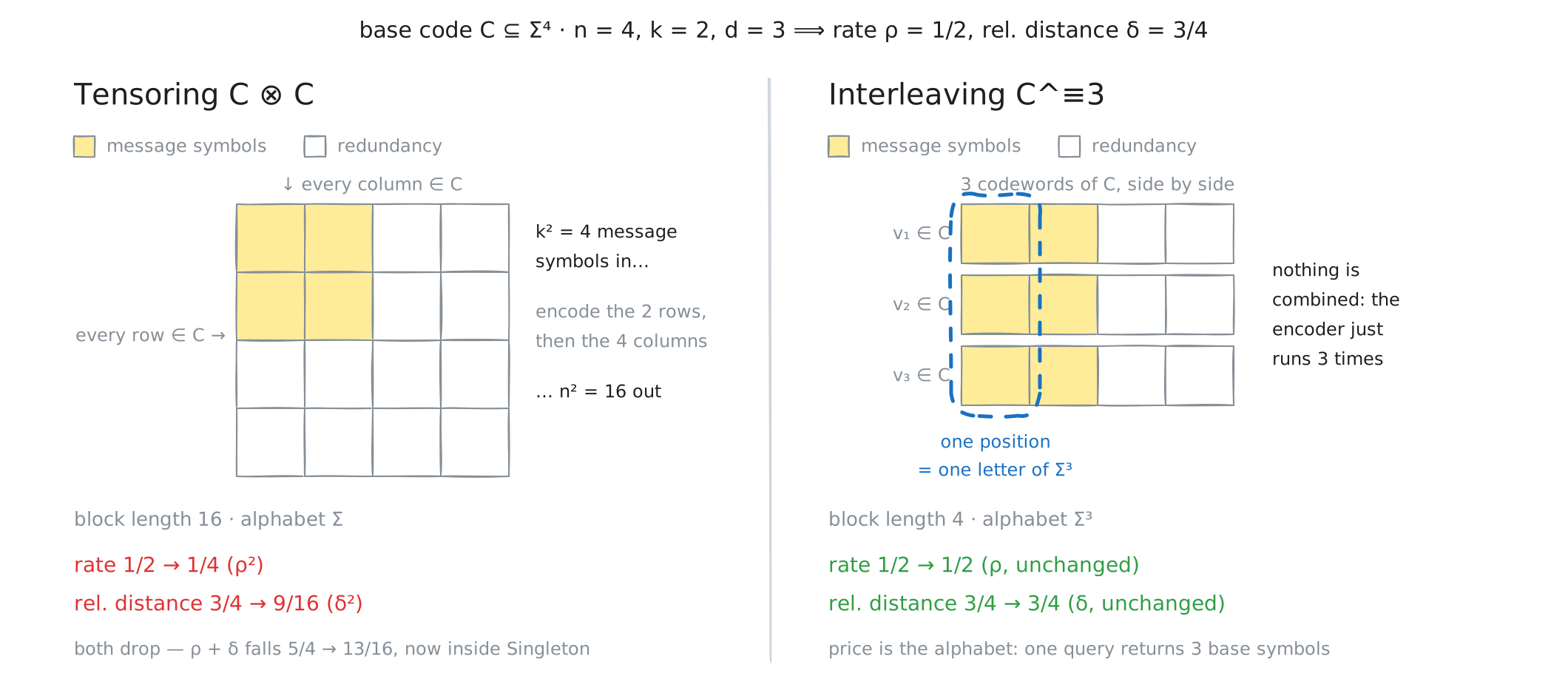
Tensoring: pay on both axes

$\mathcal C \otimes \mathcal C$ is the set of $4 \times 4$ matrices whose every row and every column is a codeword of $\mathcal C$:

How you build one. Start with a $2 \times 2$ block of message symbols. Encode each of its 2 rows with $\mathcal C$ → a $2 \times 4$ array. Then encode each of the 4 columns with $\mathcal C$ → the full $4 \times 4$. Columns are codewords by construction. Rows still are too: column-encoding applies one fixed linear map down each column, so every output row is a fixed linear combination of the two input rows, and $\mathcal C$ is linear.

Why rate squares. Read the shapes off that construction: $k^2 = 4$ message symbols went in, $n^2 = 16$ symbols came out. Rate $= k^2/n^2 = \rho^2 = 1/4$.

Why distance squares. Take any nonzero $M \in \mathcal C \otimes \mathcal C$. Some column of it is nonzero — and that column is a nonzero codeword of $\mathcal C$, so it has $\geq d$ nonzero entries. Each of those entries sits in a distinct row, so $\geq d$ rows of $M$ are nonzero. Each such row is itself a nonzero codeword, contributing $\geq d$ nonzero entries. Total $\geq d^2 = 9$ nonzero entries out of $n^2 = 16$. Relative distance $\delta^2 = 9/16$, down from $3/4$. Tight, too — the outer product $v \cdot w^\top$ of two minimum-weight codewords hits exactly $d^2$.

The catch: those are two independent losses, not a trade. $\rho + \delta$ went from $5/4$ down to $13/16 < 1$ — the tensor code is strictly inside the Singleton bound now. Concretely: at block length 16 and dimension 4, a plain RS code gets $\delta = 13/16$. The tensor code gets $9/16$ at the same rate. You paid a longer codeword and handed the adversary more room, for structure.

Interleaving: pay in alphabet

The $3$-interleaving $\mathcal C^{\equiv 3} \subseteq (\Sigma^3)^4$ stacks three codewords $v_1, v_2, v_3 \in \mathcal C$ and reads them column-wise:

Length-4 word, but each “letter” is now a triple over $\Sigma$. Nothing was combined — three codewords travel in parallel and a “position” means all three at once.

Why rate is unchanged. $3k = 6$ message symbols over $\Sigma$ in, $3n = 12$ out. Rate $= 3k/3n = \rho = 1/2$. Interleaving replicates the encoder; replication doesn’t change the payload fraction.

Why relative distance is unchanged. A position of $u$ is nonzero iff any of the three stacked codewords is nonzero there. If $u \neq 0$ then some $v_i \neq 0$, and that $v_i$ alone already forces $\geq d = 3$ nonzero positions. So $d(\mathcal C^{\equiv 3}) \geq d$ — and taking $v_1$ minimum-weight with $v_2 = v_3 = 0$ shows it’s exactly $d$. Block length is still 4, so $\delta = 3/4$, untouched.

The price is the alphabet. $\Sigma \to \Sigma^3$, and in general $\Sigma \to \Sigma^K$. One query to an interleaved codeword returns $K$ base symbols, whether or not you wanted them — so a $q$-query test costs $qK$ base-alphabet symbols. That’s what “precludes query-optimal IOPs” means: you cannot get the per-query cost below $K$.

Side by side

The two consequences that matter downstream:

• Tensoring opens up local testability and tensor sumchecks — there is structure on both axes to interrogate. This is the world TensorSwitch lives in. But the base code has to be good enough to survive squaring, and encoding is slower ($n + k$ encoder calls instead of one).
• Interleaving leaves $(\rho, \delta)$ alone, so it works for every code with no parameter slack required. Encoding is $K$ independent calls — embarrassingly parallel, and streamable in small space since you never hold more than one base codeword.

The WHIR/Ligerito family lives in the interleaving world, and so does this paper. “Works for every code” is exactly the code-agnostic promise we want to keep — and the alphabet blowup, which looks like pure cost here, turns out to be a soundness lever later: the $K$ symbols a query returns share a position, and that correlation is what keeps the list-decoding union bound from exploding, in §“The HVZK sumcheck reduction”.

Zero-knowledge encodings: the foundational object

Why plain codes leak

A plain linear-code encoding is deterministic: one message in, one codeword out. Look at three coordinates of the codeword, you’ve learned three linear functions of the message. Look at enough coordinates, you can reconstruct the message exactly. That’s the entire story of why WHIR-style proximity testing leaks — the verifier’s spot checks are reading positions of a codeword that’s a fixed function of the witness, and you can’t peek at the witness “a little bit” without peeking at it.

The fix, intuitively

Make the encoding randomized. Now the same message produces many different codewords — one per choice of fresh encoder randomness. The encoder picks one at random and sends it. The promise we want: anyone reading a few coordinates of the sent codeword should learn nothing about the underlying message. Every plausible message had a way to land on those exact coordinates, so the coordinates the verifier sees are consistent with anyone’s witness.

Think of it as a one-time pad with a budget. You can hide up to $t$ coordinates by spending enough random coins on the encoding. Beyond $t$, message structure starts showing through. The number $t$ is a parameter of the encoding — exactly the number of “free” reads the verifier is allowed without learning anything.

The smallest possible example

The mechanics fall out in the tiniest Reed–Solomon case. One message coefficient $m$, one random coefficient $r$. The encoder treats $(m, r)$ as a polynomial

and evaluates $p$ at fixed nonzero points $x_1, x_2, \dots, x_n$. The codeword is $(p(x_1), p(x_2), \dots, p(x_n))$. Now look at any single output coordinate:

Since $r$ is uniform over $\mathbb F$ and $x_i$ is a fixed nonzero scalar, $r \cdot x_i$ is uniform, and $p(x_i)$ — the value the verifier sees — is uniform too. The message $m$ contributes a constant shift, but the random coin $r$ has already smeared everything across $\mathbb F$. One coordinate, perfectly hidden.

Two coordinates is more interesting, because $r$ links them: $p(x_i) - p(x_j) = r \cdot (x_i - x_j)$. The verifier can subtract them to recover $r$, then back out $m$. So $t = 1$ is the budget with this small encoding.

Scaling up: hiding $t$ coordinates

Want $t$ hidden coordinates instead of one? Spend $t$ coins. Take $r \geq t$ fresh random field elements $\boldsymbol r$, stack them on top of the message coefficients $\boldsymbol m$, and encode the whole thing:

degree $\ell + r - 1$, evaluated at distinct nonzero $x_1, \dots, x_n$. The one-coordinate example was this with $\ell = r = 1$.

The counting, first. $p$ has $\ell + r$ coefficients, so $\ell + r$ evaluations determine it outright — and then $\boldsymbol m$ is yours. That budget splits cleanly: the $r$ coins absorb the first $r$ reads, and the remaining $\ell$ are what pin down the $\ell$ message coefficients. So $t \leq r$ ought to be free and $t > r$ ought to leak. The rest of this section makes that exact.

What we have to show is that for any query set $S$ of size $t$, the tuple $(p(x_i))_{i \in S}$ is uniform over $\mathbb F^t$ jointly — not coordinate-by-coordinate, since two individually-uniform values can still satisfy a relation that pins down $\boldsymbol m$, which is how the $\ell = r = 1$ encoding died at two queries.

Reading is affine in the coins. Fix $\boldsymbol m$ and expand a single read, multiplying the $X^{\ell}$ through:

Read that as: a constant, plus a fixed row of $r$ numbers dotted with the coin vector. The row belongs to the query — it’s $(x_i^{\ell}, x_i^{\ell+1}, \dots, x_i^{\ell+r-1})$, computable by anyone who knows $x_i$. Now write one such row per queried position and stack them. That stacking is all “collect over $S$” meant, and it turns the $t$ reads into a single matrix equation:

One row per query, one column per coin — so $M$ is $t \times r$ by construction, and entry $(i,j)$ says how much coin $j$ moves read $i$. The worked example below is literally this: $\ell = 1$, $r = 2$, queries at $x = 1, 2$ give rows $(1^1, 1^2) = (1,1)$ and $(2^1, 2^2) = (2,4)$.

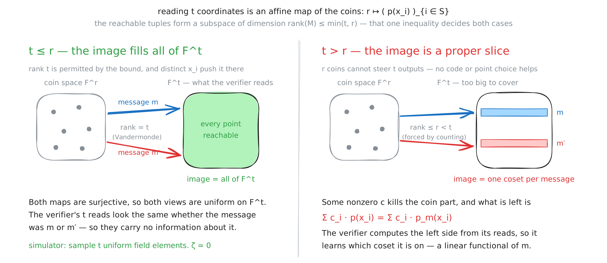
Where rank comes in. As $\boldsymbol r$ ranges over all of $\mathbb F^r$, the product $M\boldsymbol r$ ranges over exactly the span of $M$‘s columns, and the $\boldsymbol m$-term only shifts that span bodily. So the reads fill $\mathbb F^t$ precisely when those columns span $\mathbb F^t$ — which is what $\mathrm{rank}(M) = t$ means. Two ceilings follow immediately, and they’re the whole story:

— at most $r$, because $r$ vectors can’t span more than $r$ dimensions; at most $t$, because the span sits inside $\mathbb F^t$.

• $t > r$: deficient, always. $\mathrm{rank}(M) \leq r < t$, so the image is a proper subspace of $\mathbb F^t$. You cannot span a $t$-dimensional space with $r < t$ vectors, and no choice of code or evaluation points changes that.
• $t \leq r$: the ceiling is $t$, and $M$ reaches it — but only because of which numbers are in it. That is the one place the code earns its keep, and it’s what Vandermonde means.

Vandermonde, in one line. A Vandermonde matrix has geometric progressions for rows, $(1, x_i, x_i^2, \dots)$, and with distinct $x_i$ a square one is invertible — a fact you already know in polynomial clothing, since a nonzero polynomial of degree $< t$ cannot vanish at $t$ distinct points. Our $M$ is exactly that, row $i$ scaled by the nonzero $x_i^{\ell}$. So for $t \leq r$ its leftmost $t \times t$ block is an invertible Vandermonde, the rows are independent, and the rank hits $t$.

Full rank is the property with teeth: every $t$-tuple the verifier might read is produced by some coin vector, for every message. Uniform coins through a surjection stay uniform, and the $\boldsymbol m$-shift doesn’t disturb that — so the reads are uniform over $\mathbb F^t$ whatever $\boldsymbol m$ is, and the simulator just samples $t$ uniform field elements. Perfect $t$-query zero-knowledge, $\zeta = 0$.

Both cases on one example. Take $\ell = 1$, $r = 2$, so $p(X) = m + r_0X + r_1X^2$, over any $\mathbb F$ with $\mathsf{char}\,\mathbb F > 3$. Querying $x = 1, 2$ is $t = 2 \leq r$, and $M$ is the $2 \times 2$ block from above:

Invertible, so whatever target $(y_1, y_2)$ you name and whatever $m$ is, exactly one coin pair hits it — the image is all of $\mathbb F^2$, and the message only relabels which coins get you there. Now add $x = 3$, making $t = 3 > r$, and take $\boldsymbol c = (3, -3, 1)$:

Both coins cancel and the message falls out in the clear. Those weights are the Lagrange coefficients for interpolating back to $X = 0$, and $p(0) = m$.

Such a $\boldsymbol c$ exists whenever $\mathrm{rank}(M) < t$ — a proper subspace is cut out by a linear relation, so some nonzero $\boldsymbol c$ kills every column of $M$ and leaves $\sum_i c_i\,p(x_i) = \sum_i c_i\,p_{\boldsymbol m}(x_i)$, computable from what was read. The reachable tuples form a coset of $M$‘s column span, the message picks which coset, and $\boldsymbol c$ reads off which one you’re on.

The cost. The codeword now carries $\ell + r$ coefficients, so you either add $r$ evaluation points to hold the rate fixed or keep $n$ and give up relative distance. Either way you pay $r$ symbols — but $r$ only has to cover the verifier’s total query budget, which grows with the security parameter and polylogarithmically in $\ell$, never linearly. So $r/\ell \to 0$, and that is one of the places the $1 + o(1)$ headline comes from.

The abstract object

That picture generalizes to any code. We work over $\mathbb F$-additive codes — codes $\mathcal C \subseteq \Sigma^m$ whose alphabet $\Sigma$ is an $\mathbb F$-linear vector space (e.g. $\Sigma = \mathbb F^\iota$). $\Sigma = \mathbb F$ recovers ordinary linear codes; the interleaved $\mathcal C^{\equiv K}$ from the previous section is $\mathbb F$-additive whenever $\mathcal C$ is. The encoding is a randomized map

taking a message and randomness to a codeword. It is a $t$-query zero-knowledge encoding with error $\zeta$ if (i) its image lies in $\mathcal C$, and (ii) for any message $\boldsymbol m$ and any index set $S \subseteq [m]$ of size $\leq t$, the distribution $\mathsf{Enc}_{\mathcal C}(\boldsymbol m, \boldsymbol r)[S]$ over fresh $\boldsymbol r \leftarrow \mathbb F^r$ can be simulated up to statistical error $\zeta$ given only $S$ — not $\boldsymbol m$.

Reed–Solomon with appended randomness hits the definition with $\zeta = 0$ (the Vandermonde argument above). [BCL22] gives linear-time-encodable instances. The construction is code-agnostic — we won’t pin down $\mathcal C$ beyond this property.

Notation throughout. Bold $\boldsymbol m$ = the message ($\ell$ field elements). Plain $f$ = its codeword: $f = \mathsf{Enc}_{\mathcal C}(\boldsymbol m, \boldsymbol r)$. The verifier sees $f$ as an oracle; the prover knows $\boldsymbol m$ and $\boldsymbol r$.

The committed sumcheck relation

What’s actually being proved

Step back. WHIR’s job — and Ligerito’s, and Blaze’s, and every other code-agnostic IOPP’s — is to convince the verifier of one shape of claim: “the message inside this codeword satisfies some specified linear constraint.” The constraint is the point of the proof; the codeword is the vehicle.

What does “a specified linear constraint” look like? Three examples worth sitting with:

• “The polynomial whose coefficients are $\boldsymbol m$ evaluates to $\mu$ at point $x$.” This is the standard polynomial-commitment opening claim. Same as $\langle \boldsymbol m, (1, x, x^2, \dots, x^{\ell-1}) \rangle = \mu$ — a polynomial evaluation is the inner product of coefficients with powers.
• “The first coefficient of $\boldsymbol m$ is $\mu$.” Same as $\langle \boldsymbol m, (1, 0, 0, \dots, 0) \rangle = \mu$.
• “The sum of $\boldsymbol m$‘s coefficients is $\mu$.” Same as $\langle \boldsymbol m, (1, 1, 1, \dots, 1) \rangle = \mu$.

All three are the same template — pick a vector, take an inner product, claim the result. Abstract it: there’s a query vector $\boldsymbol v \in \mathbb F^\ell$ that says which question is being asked, and a claimed answer $\mu \in \mathbb F$. The protocol’s job is to convince the verifier that the secret message $\boldsymbol m$ inside the codeword satisfies $\langle \boldsymbol m, \boldsymbol v \rangle = \mu$.

$\boldsymbol v$ is the question. $\mu$ is the answer. That’s all $\boldsymbol v$ does. Different $\boldsymbol v$ = different question.

The natural relation

Translate that into an IOR-shaped relation. Verifier sees the question $\boldsymbol v$ and the claimed answer $\mu$ in the clear (explicit instance); has oracle access to a codeword $f$ (implicit instance); the prover knows the actual message and randomness:

Call this $\bar{\mathcal R}_{\mathcal C}$. Fine starting point. Leaks twice.

Leak 1: the question $\boldsymbol v$ is too big to read. $\boldsymbol v$ is $\ell$ field elements; a verifier that reads it runs in time $\Omega(\ell)$. We want polylog. The question itself has to be encoded succinctly.

Leak 2: the answer $\mu$ leaks the message. Even if the encoding $\mathsf{Enc}_{\mathcal C}$ is perfectly zero-knowledge — so $f$ leaks nothing — sending $\mu = \langle \boldsymbol m, \boldsymbol v \rangle$ in the clear leaks one linear projection of $\boldsymbol m$. That’s a real witness leak, and the protocol is going to want to talk about $\mu$ in the clear.

The paper resolves both with two modifications.

Modification 1 — succinct linear forms

Intuition. The first example of $\boldsymbol v$ above — the vector of powers $(1, x, x^2, \dots)$ — has $\ell$ entries, but it’s described by a single field element $x$. You don’t need to write the vector down; you can generate it from $x$ as needed. That’s the move: instead of letting $\boldsymbol v$ live in the explicit instance as a flat $\ell$-long blob, let the explicit instance be a small description of $\boldsymbol v$ — call it a state $\mathsf{st}$ — together with a fixed function $\mathsf{sl}$ (a “succinct linear form”) that knows how to unpack the state into the full $\boldsymbol v$ when needed.

Formally: replace $\boldsymbol v$ in the relation with $\boldsymbol v = \mathsf{sl}(\mathsf{st})$, where $\mathsf{st}$ is small. The verifier never reads $\boldsymbol v$ entry-by-entry; it only ever needs to evaluate folds of $\boldsymbol v$ (sumcheck reductions act on $\boldsymbol v$ via this fold operation), and a fold of a succinct linear form is itself computable from $\mathsf{st}$ in polylog time, following the WHIR recipe.

Anchor example. $\mathsf{sl}(\alpha) := (\alpha^{i-1})_{i \in [\ell]}$. State is the single field element $\alpha$, $\boldsymbol v$ is the vector of powers of $\alpha$, and the constraint $\langle \boldsymbol m, \boldsymbol v \rangle = \mu$ reads “the polynomial with coefficients $\boldsymbol m$ evaluates to $\mu$ at $\alpha$.” This particular form is closely related to the sumcheck-style succinct constraints in WHIR; the two are formally incomparable but both work for our purposes.

Modification 2 — masks in the constraint

Intuition. The answer $\mu$ is leaky because $\mu = \langle \boldsymbol m, \boldsymbol v \rangle$ is exactly a linear projection of the message. Stare at $\mu$, you’ve stared at one bit of the witness.

The fix is the standard zero-knowledge move: add noise. Have the prover commit to a fresh random mask and sneak the mask’s contribution into the answer. The verifier now sees $\mu' = \langle \boldsymbol m, \boldsymbol v \rangle + (\text{mask contribution})$; the prover knows both pieces; the verifier sees only the sum and can’t separate them. The mask absorbs the leak.

Where the mask comes from. The prover, before any of this gets sent to the verifier, samples small uniformly random vectors $\boldsymbol \xi_1, \dots, \boldsymbol \xi_n \in \mathbb F^{\ell_{\mathsf{zk}}}$ — one mask per “slot” we want to hide, each just a tiny block of fresh field-element noise. “Small” means $\ell_{\mathsf{zk}}$ is way shorter than $\ell$; these are nothing compared to the witness message $\boldsymbol m$.

To make these masks committable — so the verifier can ask questions about them without learning them — encode each $\boldsymbol \xi_i$ under a separate $\mathbb F$-additive code $\mathcal C_{\mathsf{zk}}$ dedicated to masks, with its own ZK encoding $\mathsf{Enc}_{\mathcal C_{\mathsf{zk}}}$. The resulting codewords $\xi_i = \mathsf{Enc}_{\mathcal C_{\mathsf{zk}}}(\boldsymbol \xi_i, \boldsymbol r_i)$ are sent to the verifier as additional oracles. Each mask comes with its own query vector $\boldsymbol u_i \in \mathbb F^{\ell_{\mathsf{zk}}}$ — same role $\boldsymbol v$ played for $\boldsymbol m$, just for the mask side.

The relation now demands a single joint constraint:

How this actually hides $\mu$. Stare at one mask term $\langle \boldsymbol \xi_i, \boldsymbol u_i \rangle$. The mask message $\boldsymbol \xi_i$ is uniform random over $\mathbb F^{\ell_{\mathsf{zk}}}$; the query vector $\boldsymbol u_i$ is fixed. The inner product of a uniform random vector with a fixed nonzero vector is itself a uniform random scalar over $\mathbb F$. So each $\langle \boldsymbol \xi_i, \boldsymbol u_i \rangle$ is a fresh uniform field element, and the sum $\sum_i \langle \boldsymbol \xi_i, \boldsymbol u_i \rangle$ is also uniform. Read the equation:

That’s a one-time pad on $\mu$. From the verifier’s view $\mu$ is a uniform field element — it could correspond to any value of the real projection, with the masks absorbing whatever offset is needed. Knowing $\mu$ leaks nothing about $\langle \boldsymbol m, \mathsf{sl}(\mathsf{st}) \rangle$.

Why the verifier can’t unmask. Reasonable worry: the verifier has oracle access to the mask codewords $\xi_i$. Could it just query them and reconstruct $\langle \boldsymbol \xi_i, \boldsymbol u_i \rangle$? No — and this is precisely why $\mathcal C_{\mathsf{zk}}$ is itself a ZK code. The same Vandermonde-style argument from §“Zero-knowledge encodings” applies: any $\leq t_{\mathsf{zk}}$ coordinates of $\xi_i$ can be simulated given only their positions, so the mask message $\boldsymbol \xi_i$ stays hidden behind the encoding the same way $\boldsymbol m$ stays hidden behind $f$. The ZK encoding on the mask side closes the loop.

Putting both modifications together gives the relation we’ll use for the rest of the article. Its data splits three ways — the standard IOR shape, made precise in §“IORs, briefly”:

Data on the left, conditions on the right: $f$ is the main oracle, the $\xi_i$ are mask oracles, both honest encodings, and the last line is the joint constraint.

That’s the committed sumcheck relation, and the table shows why it needs a protocol: the constraint is about $\boldsymbol m$ and the $\boldsymbol \xi_i$, which live in $\mathsf{w}$. The verifier has $\mathsf{x}$ in the clear and $\mathsf{y}$ only as oracles, so evaluating the constraint directly is exactly what it cannot do.

The “committed” in committed sumcheck relation is doing real work: the implicit instance $\mathsf{y} = (f, (\xi_i))$ behaves like a commitment to the message and the masks at the same time. Future protocols will accumulate more claims about this joint object; the masks travel with the protocol as oracles rather than being committed-and-opened once. Hold that thought — it’s the central design decision that makes the sumcheck step work later.

Composable HVZK for IORs (and the counterexample that forces it)

The whole construction is “compose small zero-knowledge pieces.” So we need a definition of zero-knowledge that survives composition. The textbook one doesn’t. Let’s see exactly how it breaks, because the fix is one of the conceptual contributions of the paper.

What HVZK asks for

The view is everything the verifier walks away with from one run — the prover’s messages, its own coins, its oracle query answers — as a distribution, not a fixed string.

A simulator is an efficient algorithm that manufactures a fake view from the public input alone, never the witness. The protocol is zero-knowledge if some simulator’s output lands within $\zeta$ of the real view. The moral: anything you could derive from the transcript, you could have derived alone — so it taught you nothing.

The simulator never runs in the protocol; exhibiting one is just how the privacy claim gets discharged. You’ve already met one — §“Scaling up” closed with “sample $t$ uniform field elements.”

Honest-verifier restricts the guarantee to verifiers that sample challenges as specified. As noted up top, Fiat–Shamir makes that restriction free.

IORs, briefly

We are working with interactive oracle reductions (IORs), not IOPs. The difference: an IOR verifier doesn’t output accept/reject — it outputs a new instance for some target relation $\mathcal R'$. The instance is split: an explicit part the next verifier receives as input, and an implicit part the next verifier receives as an oracle. So an IOR from $\mathcal R$ to $\mathcal R'$ takes $(\mathsf{x}, \mathsf{y}, \mathsf{w}) \in \mathcal R$ and produces $(\mathsf{x}', \mathsf{y}', \mathsf{w}') \in \mathcal R'$ via an interaction. Composition stitches IORs end-to-end: $\mathsf{IOR}_1 \circ \mathsf{IOR}_2$ runs the first reduction, then runs the second on its output.

This is the right abstraction for our purposes because the WHIR/Ligerito construction is a tower of reductions: sumcheck reduces interleaving to base, code-switching reduces big code to small code, repeat, finally land in a tiny instance you can check directly.

Where the standard definition looks — and where it doesn’t

For a protocol ending in accept/reject, §“What HVZK asks for” is the whole story. An IOR doesn’t end: its verifier outputs a new instance, part of which is an oracle handed to whatever runs next.

The standard definition audits the queries this verifier made, and says nothing about the oracle passed on. That leaves somewhere to hide a leak — an oracle nobody has queried yet.

The counterexample

Let $\mathcal R$ be any relation and $\mathcal R'$ be “check membership in $\mathcal R$ directly” — same instances, empty witness slot. Two reductions:

• $\mathsf{IOR}_1$. Prover sends the witness $\mathsf{w}$ as an oracle. Verifier queries nothing, then outputs $(\mathsf{x}', \mathsf{y}') := (\mathsf{x}, \mathsf{w})$. Complete and sound, and its view is empty — so a simulator that outputs nothing matches it perfectly. HVZK.
• $\mathsf{IOR}_2$. Prover sends nothing. Verifier reads all of $\mathsf{y}'$ and checks $(\mathsf{x}', \mathsf{y}') \in \mathcal R$. Also HVZK: the standard definition hands the simulator the same oracle access the verifier has, so it reproduces that view exactly.

Each clears the bar. Now compose: $\mathsf{IOR}_1$‘s output oracle is $\mathsf{w}$, and $\mathsf{IOR}_2$ reads it in full. The composed verifier learns the witness.

Neither piece cheats. The leak lives in the seam: $\mathsf{IOR}_1$ is graded on queries it never makes, and $\mathsf{IOR}_2$ is graded on an oracle it is handed and told is fine.

The fix — put the future queries in the definition

If the danger is what happens to the output oracle later, then later has to be part of the definition. Model “whatever will query my output oracle” as an algorithm $\mathcal D$ — a distinguisher, so called because it is the thing trying to tell a real view from a simulated one.

The simulator must now produce the view and answer $\mathcal D$‘s queries into the output oracle, still without the witness:

$\mathsf{S}$ may run $\mathcal D$ as a black box — execute it on the output instance to see which positions it wants, then invent consistent answers.

Does it kill the counterexample? Take $\mathcal D$ that reads the whole output oracle, exactly what $\mathsf{IOR}_2$ does. Now $\mathsf{IOR}_1$‘s simulator has to produce every position of $\mathsf{y}' = \mathsf{w}$ knowing only $\mathsf{x}$ — that is the witness, so it cannot. $\mathsf{IOR}_1$ now fails, which is the verdict we wanted. And when $\mathcal D$ queries nothing, it collapses back to the standard definition.

In practice $\mathcal D$ is pinned to a class: $\mathfrak D^{\leq t}$, distinguishers making at most $t$ queries to the implicit instance.

Composition — which $\mathcal D$ do you pick?

Every IOR is now HVZK only relative to some $\mathcal D$. Which one? The one that actually shows up next.

Composition theorem (Lemma 2.6 of the paper). If $\mathsf{IOR}_2$ is HVZK with respect to $\mathcal D_2$ with simulator $\mathsf{S}_2$, and $\mathsf{IOR}_1$ is HVZK with respect to $\mathcal D_1 := \mathsf{S}_2$ (running with its own distinguisher $\mathcal D_2$), then $\mathsf{IOR}_1 \circ \mathsf{IOR}_2$ is HVZK with respect to $\mathcal D_2$, with errors adding: $\zeta_1 + \zeta_2$.

Read $\mathcal D_1 := \mathsf{S}_2$ slowly, because it is the whole idea: the next protocol’s simulator becomes the previous protocol’s distinguisher. In the simulated world, $\mathsf{S}_2$ is the only thing that ever touches $\mathsf{IOR}_1$‘s output oracle — so those are the only future queries $\mathsf{IOR}_1$ has to survive. The statistical errors chain along the seam and add.

Each reduction we build is then proved HVZK against a bounded query class matching what the next stage will ask — the framework’s contribution being that “what happens to this oracle later” gets written down instead of assumed.

The HVZK sumcheck reduction

Now the first of the two key technical contributions: an HVZK reduction from testing the interleaving of a code to testing the base code itself. It is what kicks the verifier’s job down from a $2^k$-blown-up alphabet to the original. It is also where this paper buys $1 + o(1)$ overhead instead of $\geq 2\times$.

The setup: interleaving via multilinear decomposition

We are going to interleave by a power-of-two factor $K = 2^k$. The trick is to define the $2^k$-interleaving directly in terms of a zero-knowledge encoding, by splitting the message into $2^k$ pieces using multilinear-polynomial structure.

Let $\mathsf{eq}(\mathsf X_1, \dots, \mathsf X_k, \mathsf Y_1, \dots, \mathsf Y_k) := \prod_{i=1}^k (\mathsf X_i \mathsf Y_i + (1 - \mathsf X_i)(1 - \mathsf Y_i))$ — the familiar equality polynomial in $k$ pairs of variables.

Given a message $\boldsymbol m \in \mathbb F^{2^k \ell}$ and randomness $\boldsymbol r \in \mathbb F^{2^k r}$, view them as $2^k$ pieces $(\boldsymbol m_{\boldsymbol b})_{\boldsymbol b \in \{0,1\}^k}$ and $(\boldsymbol r_{\boldsymbol b})_{\boldsymbol b \in \{0,1\}^k}$, indexed by the boolean hypercube of side $k$. The interleaved encoding $\mathsf{Enc}_{\mathcal C^{\equiv 2^k}}(\boldsymbol m, \boldsymbol r)$ separately encodes each piece under $\mathsf{Enc}_{\mathcal C}$ and stacks the results:

The multilinear interpretation: if you view $\boldsymbol m$ and $\boldsymbol r$ as multilinear polynomials $\hat{\boldsymbol m}, \hat{\boldsymbol r}$ in $k + \log \ell$ and $k + \log r$ variables respectively, the first $k$ variables index which “piece” you’re in, and the remaining variables index inside the piece.

Interleaved folding

The other half of the trick: how to fold an interleaved codeword. The interleaved fold of a function $f \colon [m] \to \Sigma^{2^k}$ at a point $\boldsymbol \gamma \in \mathbb F^k$ outputs a function $[m] \to \Sigma$ defined by

where $f_{\boldsymbol b}(z) \in \Sigma$ is the $\boldsymbol b$-th coordinate of the $\Sigma^{2^k}$-vector $f(z)$. Concretely, the verifier folds an interleaved codeword by taking the $\mathsf{eq}$-weighted combination of its $2^k$ coordinates at every position.

The construction is set up so the natural identity holds:

Claim (encode-then-fold = fold-then-encode). For every message $\boldsymbol m$, randomness $\boldsymbol r$, and folding point $\boldsymbol \gamma \in \mathbb F^k$, $\mathsf{Fold}\big(\mathsf{Enc}_{\mathcal C^{\equiv 2^k}}(\boldsymbol m, \boldsymbol r),\, \boldsymbol \gamma\big) \;=\; \mathsf{Enc}_{\mathcal C}\big(\mathsf{Fold}(\boldsymbol m, \boldsymbol \gamma),\, \mathsf{Fold}(\boldsymbol r, \boldsymbol \gamma)\big).$

In English: folding the interleaved codeword gives you a valid base-code codeword whose message is the fold of the original messages. The prover folds messages, the verifier folds codewords, and the two stay in sync. This is a direct extension to zero-knowledge codes of the folding identities used in WHIR, STIR, and Ligerito.

The reduction, operationally

We have an instance of $\mathcal R_{\mathcal C^{\equiv 2^k}, \mathcal C_{\mathsf{zk}}, \mathsf{sl}}$: a $2^k$-interleaved main oracle $f$, $n$ small mask oracles $(\xi_i)$, and a joint constraint with target $\mu$. The reduction outputs an instance of $\mathcal R_{\mathcal C, \mathcal C_{\mathsf{zk}}, \mathsf{sl}'}$ — same shape, but over the base code $\mathcal C$, with a new succinct linear form $\mathsf{sl}'$ that encodes the fold.

Operationally:

After this single reduction, the problem size has dropped from $2^k \cdot m$ alphabet symbols to $m$ — the size of one base codeword.

The point — small masks, not a full mask

This is where $1 + o(1)$ overhead is won. Prior zero-knowledge sumchecks ([CFS17], [BCL22], the binary-field variant [Dia25]) add a full random polynomial of the same size as the message, then prove the original claim relative to it via a random linear combination. That doubles prover work — every operation has to be done on a $2\times$-sized object. It’s a clean construction; it’s also too expensive for our setting.

This paper does it differently: one small mask per sumcheck round, à la [XZZPS19], instead of a single full mask up front. Each mask’s message is only $\ell_{\mathsf{zk}}$ field elements (much smaller than $\ell$, the actual message size), and its encoding a correspondingly short codeword. With $k$ rounds and $\ell_{\mathsf{zk}} \ll \ell$, the total masking overhead is sublinear — exactly the $o(1)$ we want.

That’s the high-level move. The non-trivial part is making it composable with the WHIR/Ligerito recursion. Three details earn their place:

• Masks travel as oracles, not opened evaluations. [XZZPS19]‘s zero-knowledge sumcheck reveals an evaluation of the mask polynomial at the end — and inside our framework that would reveal an evaluation of $\hat{\boldsymbol m}$, breaking ZK. We cannot afford that. Instead, the reduction accumulates a claim about the masks into the next relation’s joint constraint and carries the mask oracles forward. This is exactly the work the “committed” part of $\mathcal R_{\mathcal C, \mathcal C_{\mathsf{zk}}, \mathsf{sl}}$ was set up to do. Without the joint constraint in the relation, this sumcheck would not compose.
• $\mathsf{char}(\mathbb F) \neq 2$. The mask $s_j$‘s contribution to round $j$‘s polynomial enters scaled by $2^{k-j}$ — the number of hypercube points it’s summed over. In characteristic 2 that factor vanishes for every round but the last, and the masks stop masking. A real instantiation constraint, but it doesn’t bite for the fields the WHIR/Ligerito family cares about (Goldilocks, BabyBear, large primes).
• Correlating queries over the larger alphabet. Round-by-round knowledge soundness wants a union bound over codewords at distance $\delta$ from the sent oracles. Naively, you’d “open up” the interleaved word $f$ into its $2^k$ base-code parts and union-bound each — leading to a union over $|\Lambda(\mathcal C, \delta)|^{2^k}$ events. That blows up the required field size to absurdity. The fix: analyze codewords relative to the interleaved codes $\mathcal C^{\equiv 2^k}$ and $\mathcal C_{\mathsf{zk}}^{\equiv n+k}$ directly. Interleaving raises a code’s list size by only a constant factor [GGR11], so the union bound stays modest. Operationally, the verifier’s queries are correlated across the $2^k$ stacked base-codewords — they all share the same position — and this correlation is the soundness lever. It also shrinks compiled argument size as a bonus, because correlated queries become a single Merkle path over the bigger alphabet rather than $2^k$ paths.

What this buys us

After running the reduction once, we have:

• Reduced testing the $2^k$-interleaving of $\mathcal C$ to testing $\mathcal C$ itself.
• Reduced problem size by a factor of $2^k$.
• Spent $\widetilde O(k \cdot \lambda)$ extra symbols on masks — sublinear in $m$.
• Preserved HVZK with respect to a bounded distinguisher class, by carrying mask oracles forward and accumulating their constraints.

The natural next move is to recursively shrink the codeword, which is the WHIR/Ligerito move. Each round takes a code, $2^k$-interleaves it, runs this sumcheck reduction to drop the interleaving, then switches to a new, smaller code and does it again. Recurse $O(\log \ell / \log\log \ell)$ times and the verifier ends up looking at something tiny enough to handle directly.

But the “switch to a new code” step is the second non-trivial piece, and naive code-switching is incompatible with zero-knowledge in two distinct ways. That’s Part 2.

Why we’re not done yet

We have, in zero-knowledge, the ability to reduce testing the interleaving of a code to testing the base code itself, at $1 + o(1)$ overhead, with composable HVZK guarantees that survive being plugged into a larger pipeline. That is half the construction.

The other half: at some point we need to stop testing $\mathcal C$ and start testing something smaller — a code with shorter message length, so that recursion actually terminates in something cheap. That’s code-switching: an IOR from a test for code $\mathcal C$ to a test for code $\mathcal C'$. WHIR uses it, Ligerito uses it, Blaze uses it. The non-ZK version is well understood; this paper had to find the ZK version.

Two things break when you try to make the standard code-switching template zero-knowledge:

• The randomness in the encoding gets in the way. The consistency check between old and new codewords assumes the codeword is a function of the message alone. With a zero-knowledge encoding it isn’t — it’s a function of the message and the randomness — and the obvious fix (encoding both into the new code) costs another $2\times$.
• Out-of-domain sampling is incompatible with privacy. WHIR’s OOD trick is what lets the protocol work in the list-decoding regime. The OOD vector forces the prover to commit to a single codeword among the possibilities — which is exactly what zero-knowledge forbids.

The resolution to both: a new gadget called a private zero-evader, and a joint OOD sample that operates on the message and fresh randomness. That, plus assembling everything into the headline corollary — an HVZK variant of WHIR/Ligerito at $1 + o(1)$ overhead — is Part 2.

References

• This paper — Chiesa, A., Fenzi, G., & Weissenberg, G. (Feb 2026). Zero-Knowledge IOPPs for Constrained Interleaved Codes.
• WHIR — Arnon, G., Chiesa, A., Fenzi, G., & Yogev, E. (2025). WHIR: Reed–Solomon Proximity Testing with Super-Fast Verification. EUROCRYPT ‘25. eprint
• Ligerito — Novakovic, A., & Angeris, G. (2025). Ligerito: A Small and Concretely Fast Polynomial Commitment Scheme. eprint 2025/1187
• STIR — Arnon, G., Chiesa, A., Fenzi, G., & Yogev, E. (2024). STIR: Reed–Solomon Proximity Testing with Fewer Queries. CRYPTO ‘24.
• Ligero — Ames, S., Hazay, C., Ishai, Y., & Venkitasubramaniam, M. (2017). Ligero: Lightweight Sublinear Arguments Without a Trusted Setup. CCS ‘17.
• BCL22 — Bootle, J., Chiesa, A., & Liu, S. (2022). Zero-Knowledge IOPs with Linear-Time Prover and Polylogarithmic-Time Verifier. EUROCRYPT ‘22.
• RW24 — Ron-Zewi, N., & Weiss, M. (2024). Zero-knowledge IOPs Approaching Witness Length. CRYPTO ‘24.
• XZZPS19 (Libra) — Xie, T., Zhang, J., Zhang, Y., Papamanthou, C., & Song, D. (2019). Libra: Succinct Zero-Knowledge Proofs with Optimal Prover Computation. CRYPTO ‘19.
• CFS17 — Chiesa, A., Forbes, M.A., & Spooner, N. (2017). A Zero Knowledge Sumcheck and its Applications. arXiv:1704.02086
• GGR11 — Gopalan, P., Guruswami, V., & Raghavendra, P. (2011). List Decoding Tensor Products and Interleaved Codes. SICOMP 40(5).
• Dia25 — Diamond, B. (2025). Zero-Knowledge Polynomial Commitment in Binary Fields. eprint 2025/1015
• TensorSwitch (companion blog) — TensorSwitch I.
• WHIR (companion blog) — WHIR.
• Spartan + SPARK (companion blogs) — Spartan, SPARK.